- Covered:
- Key Terms:
- sampling, sample-and-hold
- quantization, analog-to-digital
- LSB
- dithering
We need to convert a signal from analog to digital, e.g. continuous to discrete. That means making both the independent and dependent variables discrete:
- We make the independent variable (e.g. time) discrete via a sample-and-hold device, which samples and holds voltage steady at given points at time, like taking a snapshot at intervals. This is called sampling.
- We make the dependent variable (e.g. voltage) discrete via an ADC, e.g. analog-to-digital converter. It essentially rounds each snapshotted voltage to a given level, e.g. quantizing it based on the number of bits used in your ADC - your bit depth. This is called quantization.
Quantization incurs error in its rounding-off process, with a max of ±0.5 least significant bit (LSB), which is fancy jargon for “the distance between quantization levels”, or just the step size (0.5 because if you go beyond that point from a level, you’ll…just be rounded up to the next level). We can measure things in terms of LSB as a sort of unit.
Quantization error can be modeled as random noise - this additive noise has a mean of zero and a standard deviation of 0.29 LSB. This means that the greater the bit depth - the more bits we use - the smaller the quantization error, and the higher the precision. We can also add this modeled noise to the underlying signal’s inherent noise by adding their variances. This can help us figure out our actual required bit depth, because it helps us determine our expected total noise per bit depth:
When faced with the decision of how many bits are needed in a system, ask two questions: (1) How much noise is already present in the analog signal? (2) How much noise can be tolerated in the digital signal?
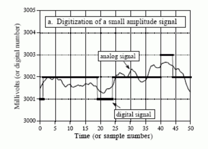
This is a powerful model, but it doesn’t hold when quantization error doesn’t appear to be random. See below for a common example - repeated quantization yields the same digital value over and over again, which doesn’t capture the actual nature of the signal (we’ve lost information!):
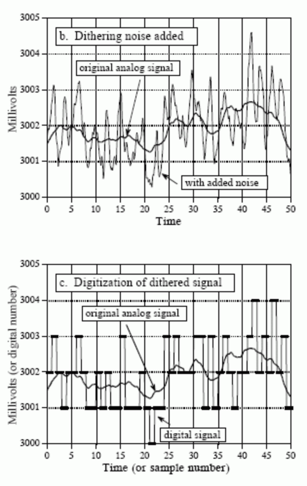
Here’s where dithering can help. Dithering adds random noise - in the given example, a normally-distributed amount with standard deviation of 2/3 LSB. This basically turns small signal fluctuations into large ones, allowing the ADC to “see” the subtleties better and digitize more accurately:
To understand how this improves the situation, imagine that the input signal is a constant analog voltage of 3.0001 volts, making it one-tenth of the way between the digital levels 3000 and 3001. Without dithering, taking 10,000 samples of this signal would produce 10,000 identical numbers, all having the value of 3000. Next, repeat the thought experiment with a small amount of dithering noise added. The 10,000 values will now oscillate between two (or more) levels, with about 90% having a value of 3000, and 10% having a value of 3001. Taking the average of all 10,000 values results in something close to 3000.1. Even though a single measurement has the inherent LSB limitation, the statistics of a large number of the samples can do much better. This is quite a strange situation: adding noise provides more information.
Visually, this looks like this:
Dithering can get quite complex (“subtractive dither”), but we don’t need to worry about that right now.