Covered:
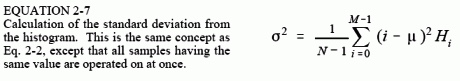
Histograms show how many times a given value has appeared. This has the effect of batching, and makes computing statistics a lot easier. So like, mean and standard deviation become:
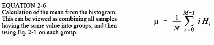
Here, H_i is the number of values that have the given value i, so like if 100 sample points had a value of 50, H_50 == 100.
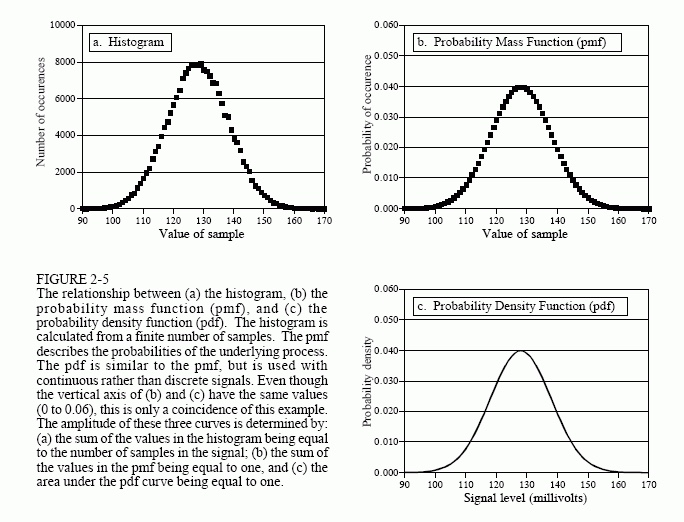
Histograms are built from acquired, measured sample points in a real signal; a probability mass function (PMF) is the function that models the underlying process that generated a given histogram. So this is all about measured - with error! - versus mathematical. The probability distribution function (PDF) is similar, but instead of being the model for discrete / digitized systems, a PDF is used for continuous signals.
As such, the y-axis of a pdf displays probability density, rather than probability - the probability of a continuous signal having exactly any one value is pretty vanishingly small. So we calculate probability from PMFs directly; we integrate between x-axis points of interest to get the probability of having a value in that range. The sum of all PMF values is 1; the integral from negative infinity to infinity of a PDF is 1.
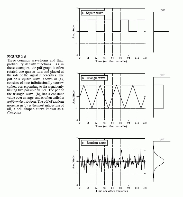
Make sure you understand how each of these signals is described by its companion PDF: